返回第二讲 · 早退与错停风险 · 网页阅读版 · 第二讲导读
什么时候值得继续计算? 固定训练好的两个出口,先预测阈值变化,再看保存的验证选择与测试错停。最简单的固定浅出口也要参加比较。
| 课堂动作 | 看哪里 | 完成什么 |
|---|---|---|
| 先读不运行 | 第 2 节三条路径账本与准确率—MAC 图 | 解释动态规则为何没有赢过固定浅出口 |
| 只改一条规则 | 第 3 节阈值练习 | 写出预期,再按验证数据重新选择 |
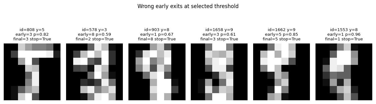
| 观察具体失败 | 错停样本图 | 区分“浅头答错”与“继续能纠正” |
数据是 sklearn digits 的 1797 张 8×8 图像,模型为 DigitsMultiExitBN-integration-20260918-lcde-r1,与主讲前面的 MNIST 机制输入不是一次连续运行。保存结果来自 2026-09-18:程序先计算两个出口,再离线回放阈值,因此 MAC 账本不是实测早退加速。
可直接读保存图;独立运行依赖 numpy torch scikit-learn matplotlib,从 load_digits() 与本册可读代码重建,不依赖另一册的 checkpoint。若顺序运行全本,会重新训练源模型并写出本地结果,课程保存输出仍用于对照。
先读这次保存运行,再作预测
先记下你的预测:动态出口是否一定比固定浅出口更划算?
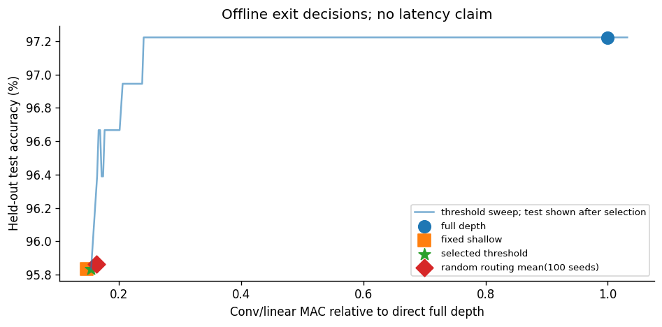
保存运行用验证集选出 τ=0.50;测试全深度 97.22%,动态 95.83%,固定浅出口也是 95.83%。动态平均 3091.73 MAC,而固定浅出口为 2944 MAC。相同准确率下,动态规则没有在这份乘加账本上占优。
随后用第 2 节的三条路径解释额外成本,再看错停:357/360 张图早退,14 张错停,其中 6 张本可由深出口纠正。验证允许下降 1 个百分点,测试下降 1.39 个百分点;留出评价并不继承验证集上的约束保证。
1. 什么在训练,什么在部署时改变?
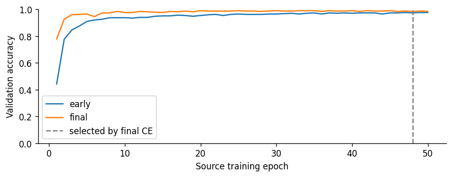
模型:输入 N×1×8×8 → Conv(1→4,3×3)+BN+ReLU+平均池化 → N×4×4×4。浅出口 flatten→10;深路径再 Conv(4→16,3×3)+BN+ReLU→flatten256→MLP32→10。两个出口一起用源标签训练 0.35 CE(early)+CE(final),50 轮中选验证集最终出口 CE 最低的 checkpoint。
这里训练参数是固定的,部署决策只选择用哪个出口的预测;与 Tent 更新 BN 参数的实验不同。固定划分约 60/20/20,分层随机按图像划分,不是按书写者隔离。测试标签不参与选 checkpoint 或选阈值。
查看代码 · 单元 4
LAB_ID='LAB13-D'

from pathlib import Path
from copy import deepcopy
import csv, hashlib, json, platform, sys, time
import numpy as np
import torch
from torch import nn
import torch.nn.functional as F
import sklearn
from sklearn.datasets import load_digits
from sklearn.model_selection import train_test_split
import matplotlib.pyplot as plt
SEED = 20260918
np.random.seed(SEED); torch.manual_seed(SEED)
torch.set_num_threads(1)
torch.use_deterministic_algorithms(True)
OUTPUT = Path('outputs') / LAB_ID
OUTPUT.mkdir(parents=True, exist_ok=True)
plt.rcParams.update({'figure.dpi':120, 'font.size':10, 'axes.spines.top':False, 'axes.spines.right':False})
def save_json(name, obj):
    (OUTPUT/name).write_text(json.dumps(obj,ensure_ascii=False,indent=2))
def save_csv(name, rows):
    with (OUTPUT/name).open('w',newline='') as f:
        w=csv.DictWriter(f, fieldnames=list(rows[0])); w.writeheader(); w.writerows(rows)
def digest_array(a): return hashlib.sha256(np.ascontiguousarray(a).tobytes()).hexdigest()
def print_table(rows, cols=None):
    cols=cols or list(rows[0]); print(' | '.join(cols)); print(' | '.join(['---']*len(cols)))
    for row in rows:
        print(' | '.join(f'{row[c]:.5f}' if isinstance(row[c],float) else str(row[c]) for c in cols))
cpu_lines=Path('/proc/cpuinfo').read_text().splitlines() if Path('/proc/cpuinfo').exists() else []
cpu_name=next((line.split(':',1)[1].strip() for line in cpu_lines if line.startswith('model name')),platform.processor())
environment={'python':sys.version.split()[0],'torch':torch.__version__,'numpy':np.__version__,
             'sklearn':sklearn.__version__,'cpu':cpu_name,'platform':platform.platform(),
             'torch_threads':torch.get_num_threads(),'device':'cpu','dtype':'float32',
             'seed':SEED,'exclusive_hardware':False}
save_json('environment.json',environment)
print(json.dumps(environment,ensure_ascii=False,indent=2))
已保存的运行输出
{
  "python": "3.12.14",
  "torch": "2.14.0+cpu",
  "numpy": "2.3.5",
  "sklearn": "1.8.0",
  "cpu": "INTEL(R) XEON(R) PLATINUM 8573C",
  "platform": "Linux-6.18.44-x86_64-with-glibc2.39",
  "torch_threads": 1,
  "device": "cpu",
  "dtype": "float32",
  "seed": 20260918,
  "exclusive_hardware": false
}
查看代码 · 单元 5
dataset = load_digits()
X = torch.tensor(dataset.images[:,None,:,:] / 16.0, dtype=torch.float32)
y = torch.tensor(dataset.target, dtype=torch.long)
all_ids = np.arange(len(y))
trainval_ids, test_ids = train_test_split(all_ids, test_size=0.2, random_state=SEED, stratify=y.numpy())
train_ids, val_ids = train_test_split(trainval_ids, test_size=0.25, random_state=SEED, stratify=y.numpy()[trainval_ids])
assert not (set(train_ids)&set(val_ids) or set(train_ids)&set(test_ids) or set(val_ids)&set(test_ids))
assert len(train_ids)+len(val_ids)+len(test_ids)==len(y)
split_manifest={'dataset':'sklearn.datasets.load_digits; 1797 real 8x8 images; pixel/16',
                'counts':{'train':len(train_ids),'validation':len(val_ids),'test':len(test_ids)},
                'train_ids':train_ids.tolist(),'validation_ids':val_ids.tolist(),'test_ids':test_ids.tolist(),
                'input_sha256':digest_array(X.numpy()),'labels_sha256':digest_array(y.numpy()),
                'split_policy':'stratified random by sample, NOT writer-disjoint', 'test_labels':'evaluation only'}
save_json('split-manifest.json',split_manifest)
print('Split:',split_manifest['counts'])
已保存的运行输出
Split: {'train': 1077, 'validation': 360, 'test': 360}
查看代码 · 单元 6
MODEL_ID = 'DigitsMultiExitBN-integration-20260918-lcde-r1'
class DigitsMultiExitBN(nn.Module):
    def __init__(self):
        super().__init__()
        self.conv1=nn.Conv2d(1,4,3,padding=1,bias=False)
        self.bn1=nn.BatchNorm2d(4)
        self.early=nn.Linear(4*4*4,10)
        self.conv2=nn.Conv2d(4,16,3,padding=1,bias=False)
        self.bn2=nn.BatchNorm2d(16)
        self.fc=nn.Linear(16*4*4,32)
        self.final=nn.Linear(32,10)
    def forward(self,x):
        h=F.avg_pool2d(F.relu(self.bn1(self.conv1(x))),2)
        early=self.early(h.flatten(1))
        h=F.relu(self.bn2(self.conv2(h)))
        final=self.final(F.relu(self.fc(h.flatten(1))))
        return early,final

def train_source():
    torch.manual_seed(SEED)
    model=DigitsMultiExitBN()
    optimizer=torch.optim.Adam(model.parameters(),lr=0.003)
    order_generator=torch.Generator().manual_seed(SEED+1)
    best_loss=float('inf'); best_state=None; best_epoch=None; history=[]
    for epoch in range(1,51):
        model.train()
        order=torch.as_tensor(train_ids)[torch.randperm(len(train_ids),generator=order_generator)]
        total=0.0
        for ids in order.split(64):
            optimizer.zero_grad(set_to_none=True)
            early,final=model(X[ids]); loss=0.35*F.cross_entropy(early,y[ids])+F.cross_entropy(final,y[ids])
            loss.backward(); optimizer.step(); total += loss.item()*len(ids)
        model.eval()
        with torch.no_grad():
            ve,vf=model(X[val_ids]); val_loss=F.cross_entropy(vf,y[val_ids]).item()
        history.append({'epoch':epoch,'train_weighted_loss':total/len(train_ids),
                        'validation_final_ce':val_loss,'validation_early_acc':(ve.argmax(1)==y[val_ids]).float().mean().item(),
                        'validation_final_acc':(vf.argmax(1)==y[val_ids]).float().mean().item()})
        if val_loss < best_loss:
            best_loss=val_loss; best_state=deepcopy(model.state_dict()); best_epoch=epoch
    model.load_state_dict(best_state); model.eval()
    return model,history,best_epoch
source_model,train_history,best_epoch=train_source()
source_state=deepcopy(source_model.state_dict())
state_hash=hashlib.sha256(b''.join(k.encode()+v.cpu().numpy().tobytes() for k,v in sorted(source_state.items()))).hexdigest()
save_csv('source-training.csv',train_history)
# Transparent JSON state is a local convenience; notebook always reconstructs from readable code.
save_json('source-state.json',{k:v.tolist() for k,v in source_state.items()})
model_manifest={'model_id':MODEL_ID,'state_sha256':state_hash,'best_epoch':best_epoch,
                'checkpoint_selection':'minimum validation final-exit CE over 50 epochs',
                'train_loss':'0.35*CE(early)+CE(final)','optimizer':'Adam lr=0.003 batch=64',
                'initialization_seed':SEED,'params':sum(p.numel() for p in source_model.parameters()),
                'old_LAB02_dependency':False,'data_split_sha256':hashlib.sha256(json.dumps(split_manifest,sort_keys=True).encode()).hexdigest()}
save_json('model-manifest.json',model_manifest)
print(json.dumps(model_manifest,indent=2))
已保存的运行输出
{
  "model_id": "DigitsMultiExitBN-integration-20260918-lcde-r1",
  "state_sha256": "544bb0f79f5759b66656565e3e4c5a59a5dd8f2893a067d93a7fe331439c685c",
  "best_epoch": 48,
  "checkpoint_selection": "minimum validation final-exit CE over 50 epochs",
  "train_loss": "0.35*CE(early)+CE(final)",
  "optimizer": "Adam lr=0.003 batch=64",
  "initialization_seed": 20260918,
  "params": 9856,
  "old_LAB02_dependency": false,
  "data_split_sha256": "6f705c12f1651f0c5b871f8ff65f4241bdbc1ffbd61a5f0fc56ac95bbb0cf129"
}
查看代码 · 单元 7
fig,ax=plt.subplots(figsize=(7.5,3))
ax.plot([r['epoch'] for r in train_history],[r['validation_early_acc'] for r in train_history],label='early')
ax.plot([r['epoch'] for r in train_history],[r['validation_final_acc'] for r in train_history],label='final')
ax.axvline(best_epoch,color='gray',linestyle='--',label='selected by final CE')
ax.set(xlabel='Source training epoch',ylabel='Validation accuracy',ylim=(0,1)); ax.legend()
fig.tight_layout(); fig.savefig(OUTPUT/'training.png'); plt.show()
with torch.inference_mode():
    val_early,val_final=source_model(X[val_ids]); test_early,test_final=source_model(X[test_ids])
for split,ids,e,f in [('validation',val_ids,val_early,val_final),('test',test_ids,test_early,test_final)]:
    rows=[]
    for i,sample_id in enumerate(ids):
        row={'sample_id':int(sample_id),'target':int(y[sample_id])}
        row.update({f'early_logit_{k}':float(e[i,k]) for k in range(10)})
        row.update({f'final_logit_{k}':float(f[i,k]) for k in range(10)})
        rows.append(row)
    save_csv(f'{split}-exit-logits.csv',rows)
print('Both exits computed and saved; no runtime early exit implemented.')
已保存的运行输出
Both exits computed and saved; no runtime early exit implemented.
Matplotlib figure
2. 阈值只在验证集选,出口开销也记账
用浅出口最大 softmax 概率作为停止分数。候选阈值 0.50–0.99;另加 1.01 表示不早退。先满足验证准确率不低于全深度基线 1 个百分点,再选期望 MAC 最低的阈值;这只是预先固定的教学决策规则,不是置信保证。
卷积/线性 MAC:block1=2304,浅头=640,block2+深头=17728。全深度直接路径为 20032;动态拒绝早退还额外付浅头,总计 20672;早退为 2944。表中包含浅出口开销,不包含 BN/激活/池化、softmax/门控/数据搬运与排队,所以叫 conv/linear MAC 代理而非完整执行成本。全深度基线跳过浅头。随机策略以验证得到的早退比例为概率,每个样本随机选择,100 个预定 seed,不据测试表现挑 seed。
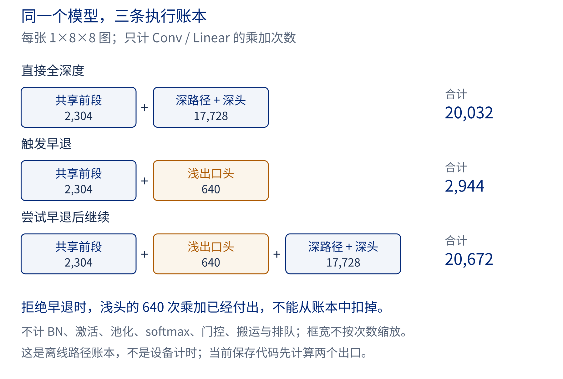
先看什么。 比较全深度与“尝试后继续”:后者多了哪一个框?再检查早退路径为什么不含深路径和深头。
改变一个条件。 提高退出阈值,更多样本选择继续。平均乘加次数与错停数量可能各怎样变化?先作预测,再按验证规则观察保存曲线。
从当前代码核对每一笔。 第一层卷积为 $8\times8\times4\times1\times3\times3=2304$;浅头为 $64\times10=640$。尾部为第二层卷积 $4\times4\times16\times4\times3\times3=9216$,加 $256\times32=8192$ 与 $32\times10=320$,合计 $17728$。BN、ReLU、池化等没有被改写成零开销,只是不属于这份 conv/linear 乘加口径。
当前保存程序先算两只出口,再离线回放规则;这些和数表示候选执行路径应付的账,不是已测运行时间。保持下方保存结果:测试集 360 张,选定动态策略与固定浅出口同为 95.83%,动态平均 3091.73 MAC 高于固定浅出口的 2944 MAC。因此这个例子里的动态规则没有在准确率与该计算账本上优于固定浅出口。
查看代码 · 单元 9
SHARED,EARLY_HEAD,TAIL=2304,640,17728
EARLY_MAC=SHARED+EARLY_HEAD
DYNAMIC_LATE_MAC=SHARED+EARLY_HEAD+TAIL
FULL_MAC=SHARED+TAIL
THRESHOLDS=np.r_[np.arange(.50,1.0,.01),1.01]
def policy(early,final,labels,threshold):
    stopped=early.softmax(1).max(1).values.numpy()>=threshold
    ep,fp=early.argmax(1).numpy(),final.argmax(1).numpy()
    pred=np.where(stopped,ep,fp); truth=labels.numpy()
    return {'threshold':float(threshold),'accuracy':float(np.mean(pred==truth)),
            'early_fraction':float(stopped.mean()),'mean_conv_linear_mac':float(np.where(stopped,EARLY_MAC,DYNAMIC_LATE_MAC).mean()),
            'wrong_early_count':int(np.sum(stopped&(ep!=truth))),
            'avoidable_wrong_early_count':int(np.sum(stopped&(ep!=truth)&(fp==truth)))},stopped,pred
val_rows=[policy(val_early,val_final,y[val_ids],t)[0] for t in THRESHOLDS]
val_full_acc=float((val_final.argmax(1)==y[val_ids]).float().mean())
feasible=[r for r in val_rows if r['accuracy']>=val_full_acc-.01]
chosen=min(feasible,key=lambda r:(r['mean_conv_linear_mac'],-r['accuracy'],-r['threshold']))
chosen_t=chosen['threshold']; random_probability=chosen['early_fraction']
save_csv('validation-thresholds.csv',val_rows)
save_json('threshold-selection.json',{'chosen':chosen,'full_validation_acc':val_full_acc,'max_validation_accuracy_drop':.01,
              'test_labels_used':False,'mac_scope':'conv/linear only; includes early head for dynamic policy; gate omitted',
              'counts':{'shared':SHARED,'early_head':EARLY_HEAD,'tail':TAIL,'direct_full':FULL_MAC}})
print('Selected using validation only:',json.dumps(chosen,indent=2))
已保存的运行输出
Selected using validation only: {
  "threshold": 0.5,
  "accuracy": 0.975,
  "early_fraction": 0.9805555555555555,
  "mean_conv_linear_mac": 3288.711111111111,
  "wrong_early_count": 7,
  "avoidable_wrong_early_count": 4
}
查看代码 · 单元 10
test_rows=[]
for t in THRESHOLDS: test_rows.append(policy(test_early,test_final,y[test_ids],t)[0])
chosen_test,stopped,pred=policy(test_early,test_final,y[test_ids],chosen_t)
ep=test_early.argmax(1).numpy(); fp=test_final.argmax(1).numpy(); truth=y[test_ids].numpy()
random_rows=[]
for seed in range(100):
    take_early=np.random.default_rng(SEED+100+seed).random(len(test_ids))<random_probability
    rp=np.where(take_early,ep,fp)
    random_rows.append({'seed':SEED+100+seed,'accuracy':float(np.mean(rp==truth)),'early_fraction':float(take_early.mean()),
                        'mean_conv_linear_mac':float(np.where(take_early,EARLY_MAC,FULL_MAC).mean())})
# Random routing is known before the early head; deep-routed samples skip early head.
summary=[{'policy':'full depth','accuracy':float(np.mean(fp==truth)),'early_fraction':0.0,'mean_conv_linear_mac':float(FULL_MAC)},
         {'policy':'fixed shallow','accuracy':float(np.mean(ep==truth)),'early_fraction':1.0,'mean_conv_linear_mac':float(EARLY_MAC)},
         {'policy':'selected threshold','accuracy':chosen_test['accuracy'],'early_fraction':chosen_test['early_fraction'],
          'mean_conv_linear_mac':chosen_test['mean_conv_linear_mac']},
         {'policy':'random routing mean(100 seeds)','accuracy':float(np.mean([r['accuracy'] for r in random_rows])),
          'early_fraction':float(np.mean([r['early_fraction'] for r in random_rows])),
          'mean_conv_linear_mac':float(np.mean([r['mean_conv_linear_mac'] for r in random_rows]))}]
save_csv('test-thresholds.csv',test_rows); save_csv('random-policies.csv',random_rows);save_csv('policy-summary.csv',summary)
rows=[{'sample_id':int(s),'target':int(truth[i]),'early_prediction':int(ep[i]),'final_prediction':int(fp[i]),
       'early_confidence':float(test_early.softmax(1)[i].max()),'stopped':bool(stopped[i]),'policy_prediction':int(pred[i])} for i,s in enumerate(test_ids)]
save_csv('selected-policy-per-sample.csv',rows)
print_table(summary)
print('Chosen policy wrong early exits:',chosen_test['wrong_early_count'],
      '; final exit would fix:',chosen_test['avoidable_wrong_early_count'])
print('Random accuracy SD over predefined seeds:',float(np.std([r['accuracy'] for r in random_rows],ddof=1)))
fig,ax=plt.subplots(figsize=(8,4))
ax.plot([r['mean_conv_linear_mac']/FULL_MAC for r in test_rows], [100*r['accuracy'] for r in test_rows],'-',label='threshold sweep; test shown after selection',alpha=.6)
for r,m in zip(summary,['o','s','*','D']):
    ax.scatter(r['mean_conv_linear_mac']/FULL_MAC,100*r['accuracy'],marker=m,s=110,label=r['policy'])
ax.set(xlabel='Conv/linear MAC relative to direct full depth',ylabel='Held-out test accuracy (%)',
       title='Offline exit decisions; no latency claim')
ax.legend(fontsize=8,loc='best');fig.tight_layout(); fig.savefig(OUTPUT/'accuracy-mac.png');plt.show()
已保存的运行输出
policy | accuracy | early_fraction | mean_conv_linear_mac
--- | --- | --- | ---
full depth | 0.97222 | 0.00000 | 20032.00000
fixed shallow | 0.95833 | 1.00000 | 2944.00000
selected threshold | 0.95833 | 0.99167 | 3091.73333
random routing mean(100 seeds) | 0.95861 | 0.98153 | 3259.65333
Chosen policy wrong early exits: 14 ; final exit would fix: 6
Random accuracy SD over predefined seeds: 0.0012793505179773243
Matplotlib figure
查看代码 · 单元 11
wrong=np.flatnonzero(stopped&(ep!=truth))
# If none exist at selected threshold, show actual high-confidence shallow errors without pretending they stopped.
show_ids=wrong[:6]
plot_label='Wrong early exits at selected threshold'
if not len(show_ids):
    errors=np.flatnonzero(ep!=truth)
    show_ids=errors[np.argsort(-test_early.softmax(1).max(1).values.numpy()[errors])[:6]]
    plot_label='No wrong selected exits; these shallow errors did NOT necessarily stop'
fig,axs=plt.subplots(1,max(1,len(show_ids)),figsize=(max(5,1.7*len(show_ids)),3.0),squeeze=False)
for ax,j in zip(axs[0],show_ids):
    ax.imshow(X[test_ids[j],0],cmap='gray',vmin=0,vmax=1);ax.axis('off')
    ax.set_title(f'id={test_ids[j]} y={truth[j]}\nearly={ep[j]} p={float(test_early.softmax(1)[j].max()):.2f}\nfinal={fp[j]} stop={bool(stopped[j])}',fontsize=8)
fig.suptitle(plot_label,fontsize=10);fig.tight_layout(rect=[0,0,1,.84]);fig.savefig(OUTPUT/'wrong-exits.png');plt.show()
已保存的运行输出
Matplotlib figure
3. 哪项结果能改变你的判断?
先核对一条路径,再解释平均值
保存测试里 357 张早退、3 张继续。用账本算:$(357\times2944+3\times20672)/360=3091.73$。这里 3 张继续的样本已经付过浅头的 640 MAC,所以不能按全深度直接路径 20032 记账。
预测题。 将阈值设为 1.01,所有样本都拒绝早退,动态路径的平均 MAC 是 20032 还是 20672?为何这与“直接全深度”不同?
核对思路。 应是 20672。每张图先算浅头再继续,额外的 640 不会因没有样本早退而消失;直接全深度基线则不需要尝试浅头。随机路由在计算浅头前已知道选择,因此它的深路径可以跳过浅头,账本也不同。
改一个规则,再用验证集选
固定模型和数据,先只把验证允许损失从 1 个百分点改为 0;另一次再把停止分数从最大概率改为概率间隔。每次先写预测、重新执行验证选择,保留原测试报告。完整测试曲线只供选择完成后解释趋势,不从里面挑“最佳阈值”冒充验证选择。
提高阈值会使早退集合收缩,但测试准确率不必单调上升:某些样本的浅头可能正确、深头反而错误。请用逐样本的两个预测解释,而不只看平均值。反复查看同一测试集已成为开发活动;正式新结论需要新的留出评价。
把计算判断变成研究设计
若要问“实际会不会更快”,还需实现真实跳过尾部,测量浅头、门控、batch 重组和延迟。先读完整教师示例与空白研究卡,只替换一个条件,再回到研究卡主讲讨论失败条件。
返回第二讲 · 早退结果比较 · 网页阅读版与保存结果 · 下载 Lecture02-LAB11.ipynb · 课程导读