LAB 09 · 视觉 Attention 完整层
返回第二讲 · 完整 Attention 选读 · 网页阅读版 · 第二讲导读
改一块图像,为什么另一块的输出也会改变? 本册是完整 Attention 的后续选读,不是本次课堂或第三讲的前置任务。
用 4×4 灰度图、四个 2×2 patch、4 维表示与双 head 走完一个 pre-norm 层:X → LN → attention → 加 X → LN → 逐 token MLP → 第二条残差。全部权重固定,没有训练和类别标签;保存张量支持核对计算,不证明学到了语义关注。
| 读法 | 从哪里开始 | 具体动作 |
|---|---|---|
| 先读保存结果 | 第 1、3、4 节的图 | 追踪被修改 patch 对其他 token 的影响 |
| 核对一行计算 | 第 3 节 | 选 head=0、query=0,手算四个 V 的加权和 |
| 独立重算 | 从第一个代码块顺序运行 | 只改一个像素或位置条件,再比较中间张量 |
本册只需 NumPy 与 Matplotlib,不依赖其他 Notebook 的运行内存。语言的因果 mask 可在 Lecture 01 · LAB05 对照阅读;这里四个图块互相可见,没有 causal mask。
1. 先作预测,再建立可复算的输入
只改右下 patch 的一个像素:你预计是一个输出 token 变,还是全部 token 都可能变?如果 4 个 token 完全相同、又没有位置差异,注意力矩阵还会偏向某个位置吗?
运行要求:Python 3.10+、NumPy、Matplotlib。若缺依赖,在 notebook 外安装 python -m pip install numpy matplotlib。重算只使用本文件代码;输出写入当前目录下 outputs/LAB-B,不会覆盖其他 Lab。
查看代码 · 单元 5
from pathlib import Path
import json, sys, platform, hashlib
import numpy as np
import matplotlib.pyplot as plt
np.set_printoptions(precision=4, suppress=True)
OUTPUT = Path('outputs/LAB-B')
OUTPUT.mkdir(parents=True, exist_ok=True)
SEED = 20260918
DTYPE = np.float64
EPS = 1e-5
plt.rcParams.update({'font.size': 11, 'figure.dpi': 120, 'axes.spines.top': False, 'axes.spines.right': False})
image = np.array([[0., 0.2, 0.8, 1.0], [0.1, 0.3, 0.7, 0.9],
                  [0.9, 0.7, 0.2, 0.1], [1., 0.8, 0.3, 0.]], dtype=DTYPE)
def patchify(im):
    # Row-major order: top-left, top-right, bottom-left, bottom-right.
    return im.reshape(2, 2, 2, 2).transpose(0, 2, 1, 3).reshape(4, 4)
patches = patchify(image)
W_patch = np.array([[1., .1, 0., -.2], [.2, .8, -.1, 0.],
                    [0., -.2, 1., .2], [-.1, 0., .1, .9]])
position = np.array([[.2, 0., 0., 0.], [0., .2, 0., 0.],
                     [0., 0., .2, 0.], [0., 0., 0., .2]])
embedded = patches @ W_patch
X = embedded + position
print('image', image.shape, 'patches', patches.shape, 'embedding', embedded.shape, 'tokens X', X.shape)
print('patch vectors:\n', patches)
print('X = patches @ W_patch + position:\n', X)
fig, ax = plt.subplots(1, 2, figsize=(9, 3.8))
a = ax[0].imshow(image, cmap='gray', vmin=0, vmax=1)
ax[0].axvline(1.5, color='#e6b450', lw=2); ax[0].axhline(1.5, color='#e6b450', lw=2)
for i, (x, y) in enumerate([(0.5, .5), (2.5, .5), (.5, 2.5), (2.5, 2.5)]):
    ax[0].text(x,y,f'P{i}',ha='center',color='#f2ab32',fontweight='bold')
ax[0].set_title('Constructed image | 4 patches')
im = ax[1].imshow(X, cmap='viridis'); fig.colorbar(im, ax=ax[1], shrink=.8)
ax[1].set(title='Projected pixels + position', xlabel='Channel', ylabel='Patch token')
fig.tight_layout(); fig.savefig(OUTPUT/'01-patches.png'); plt.show()
保存输出 · 2026-09-18 本地逐单元计算,非 Deepnote 云端运行
image (4, 4) patches (4, 4) embedding (4, 4) tokens X (4, 4)
patch vectors:
 [[0.  0.2 0.1 0.3]
 [0.8 1.  0.7 0.9]
 [0.9 0.7 1.  0.8]
 [0.2 0.1 0.3 0. ]]
X = patches @ W_patch + position:
 [[0.21 0.14 0.11 0.29]
 [0.91 0.94 0.69 0.79]
 [0.96 0.45 1.21 0.74]
 [0.22 0.04 0.29 0.22]]
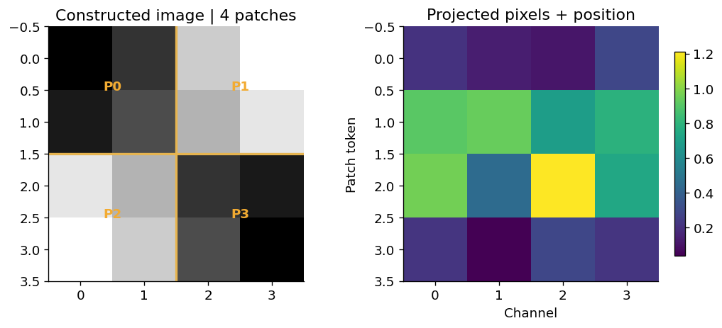
位置向量只是按 token 加进去的固定数;它不是从图片推断的坐标。此处 4 个 patch 都保留,没有 class token 或最终分类头。W_patch 和后面所有权重都是固定教学权重。
2. 完整层的约定
每个 token 独立做 LayerNorm:按它自己的 4 个通道求均值、方差;gamma=1, beta=0, epsilon=1e-5。每个 head 的维度 d_k=d_v=2,因此分数除以 sqrt(2),再沿被读取的 key 轴做 softmax。
Q,K,V 都来自第一个 LayerNorm 的输出。每个 head 读回的 V 拼接后经过 W_O,才与原始 X 相加。第二个 LN 的结果经过同一套逐 token MLP(4→6→4、GELU),最后与第一条残差的结果相加。dropout 关闭;本例没有 bias,LN affine 取恒等。
先核对维度,再看数字。否则很容易把“各位置交换信息”与“每个位置变换通道”混为一谈。
查看代码 · 单元 10
D, HEADS, DH, DFF = 4, 2, 2, 6
rng = np.random.default_rng(SEED)
weights = {name: rng.normal(0, .35, shape).astype(DTYPE) for name, shape in [
    ('W_Q', (D,D)), ('W_K', (D,D)), ('W_V', (D,D)), ('W_O', (D,D)),
    ('W_1', (D,DFF)), ('W_2', (DFF,D))]}
def ln(x):
    return (x-x.mean(axis=-1,keepdims=True))/np.sqrt(x.var(axis=-1,keepdims=True)+EPS)
def softmax(x):
    e = np.exp(x-x.max(axis=-1,keepdims=True))
    return e/e.sum(axis=-1,keepdims=True)
def gelu(x):
    # The tanh approximation is declared explicitly; no library default ambiguity.
    return .5*x*(1+np.tanh(np.sqrt(2/np.pi)*(x+.044715*x**3)))
def encoder(x):
    t = {'input': x.copy(), 'ln1': ln(x)}
    for name in ('Q','K','V'):
        t[name] = t['ln1'] @ weights['W_'+name]
        t[name+'_heads'] = t[name].reshape(len(x),HEADS,DH).transpose(1,0,2)
    t['scores'] = t['Q_heads'] @ t['K_heads'].transpose(0,2,1) / np.sqrt(DH)
    t['attention'] = softmax(t['scores'])
    t['read_values'] = t['attention'] @ t['V_heads']
    t['concat'] = t['read_values'].transpose(1,0,2).reshape(len(x),D)
    t['projected_attention'] = t['concat'] @ weights['W_O']
    t['residual1'] = x + t['projected_attention']
    t['ln2'] = ln(t['residual1'])
    t['mlp_hidden_pre'] = t['ln2'] @ weights['W_1']
    t['mlp_hidden'] = gelu(t['mlp_hidden_pre'])
    t['mlp_output'] = t['mlp_hidden'] @ weights['W_2']
    t['output'] = t['residual1'] + t['mlp_output']
    return t
trace = encoder(X)
for name, value in trace.items(): print(f'{name:22s} {str(value.shape):14s}')
print('Head 0 attention weights (row=query, column=key):\n', trace['attention'][0])
print('Head 0 read-back values:\n', trace['read_values'][0])
print('Final output:\n', trace['output'])
保存输出 · 2026-09-18 本地逐单元计算,非 Deepnote 云端运行
input                  (4, 4)
ln1                    (4, 4)
Q                      (4, 4)
Q_heads                (2, 4, 2)
K                      (4, 4)
K_heads                (2, 4, 2)
V                      (4, 4)
V_heads                (2, 4, 2)
scores                 (2, 4, 4)
attention              (2, 4, 4)
read_values            (2, 4, 2)
concat                 (4, 4)
projected_attention    (4, 4)
residual1              (4, 4)
ln2                    (4, 4)
mlp_hidden_pre         (4, 6)
mlp_hidden             (4, 6)
mlp_output             (4, 4)
output                 (4, 4)
Head 0 attention weights (row=query, column=key):
 [[0.1624 0.1705 0.3532 0.314 ]
 [0.3184 0.3073 0.179  0.1953]
 [0.0366 0.044  0.554  0.3655]
 [0.0378 0.0452 0.5511 0.3659]]
Head 0 read-back values:
 [[-0.3022 -0.0763]
 [-0.0288 -0.1743]
 [-0.5419  0.0128]
 [-0.5396  0.0118]]
Final output:
 [[-0.5644  0.4532  0.0506 -0.1394]
 [ 0.6503  0.9269  0.6401  0.332 ]
 [-0.0476  1.3125  1.3218  0.9238]
 [-0.7901  0.6609  0.2428  0.0266]]
中间数值表:先查看,再独立核对一行
下面列出投影、缩放后的分数和完整层两条分支。全表也写入 results.json 与 tensors.npz,因此可以在不截屏、不复制舍入数字的情况下核算。手算时选择一个 query、一个 head 即可;不要把四位小数的显示误差当成模型差异。
查看代码 · 单元 14
for name in ['ln1','Q','K','V','scores','concat','projected_attention','residual1','ln2','mlp_hidden_pre','mlp_hidden','mlp_output','output']:
    print(name, trace[name].shape)
    print(trace[name])
保存输出 · 2026-09-18 本地逐单元计算,非 Deepnote 云端运行
ln1 (4, 4)
[[ 0.3238 -0.6836 -1.1153  1.475 ]
 [ 0.7778  1.0789 -1.4301 -0.4265]
 [ 0.4287 -1.3932  1.3218 -0.3572]
 [ 0.2969 -1.6465  1.0527  0.2969]]
Q (4, 4)
[[-0.2322  0.3838 -0.0612 -0.4661]
 [ 0.1665 -0.302  -0.4704  0.13  ]
 [-0.9418  0.9437  0.6336  0.2455]
 [-0.9088  0.9923  0.6176  0.0188]]
K (4, 4)
[[ 1.4217 -0.5779  0.3854  1.3568]
 [ 1.1773 -0.5467 -0.4739  0.3812]
 [-1.6563  0.4223  0.7644 -0.8131]
 [-1.1733  0.281   0.8805 -0.3077]]
V (4, 4)
[[ 0.0894 -0.4812  0.5537 -0.7136]
 [ 0.5686 -0.0902 -0.7087 -0.0763]
 [-0.6207  0.1009  1.0437  0.0813]
 [-0.6192 -0.0587  1.2253 -0.1574]]
scores (2, 4, 4)
[[[-0.3903 -0.3417  0.3866  0.2689]
  [ 0.2908  0.2553 -0.2851 -0.1981]
  [-1.3324 -1.1489  1.3848  0.9688]
  [-1.3192 -1.1402  1.3607  0.9512]]

 [[-0.4638 -0.1051  0.2349  0.0633]
  [-0.0034  0.1927 -0.329  -0.3212]
  [ 0.4082 -0.1462  0.2013  0.3411]
  [ 0.1864 -0.2019  0.323   0.3804]]]
concat (4, 4)
[[-0.3022 -0.0763  0.6052 -0.1509]
 [-0.0288 -0.1743  0.3646 -0.2352]
 [-0.5419  0.0128  0.6444 -0.2524]
 [-0.5396  0.0118  0.6827 -0.2138]]
projected_attention (4, 4)
[[-0.3659  0.2188 -0.0172  0.1302]
 [-0.156   0.0641 -0.0012 -0.0502]
 [-0.4727  0.3029  0.0235  0.3042]
 [-0.4889  0.3132  0.011   0.2995]]
residual1 (4, 4)
[[-0.1559  0.3588  0.0928  0.4202]
 [ 0.754   1.0041  0.6888  0.7398]
 [ 0.4873  0.7529  1.2335  1.0442]
 [-0.2689  0.3532  0.301   0.5195]]
ln2 (4, 4)
[[-1.461   0.7845 -0.376   1.0525]
 [-0.3492  1.6971 -0.8825 -0.4654]
 [-1.3815 -0.4459  1.2471  0.5803]
 [-1.6668  0.4275  0.2518  0.9874]]
mlp_hidden_pre (4, 6)
[[ 0.939  -0.0917 -0.3395  1.4627  0.3768  0.1692]
 [-1.4072 -0.6563 -1.5472  0.7997  0.2691  0.0457]
 [ 1.6753  0.6078  0.3688  1.1938 -0.3456  0.0579]
 [ 1.3559  0.1787 -0.1395  1.6026  0.1249  0.1478]]
mlp_hidden (4, 6)
[[ 0.7756 -0.0425 -0.1246  1.3575  0.2437  0.0959]
 [-0.1124 -0.1679 -0.0944  0.6302  0.1631  0.0237]
 [ 1.5966  0.4426  0.2374  1.0547 -0.1261  0.0303]
 [ 1.2369  0.102  -0.062   1.5151  0.0687  0.0826]]
mlp_output (4, 4)
[[-0.4085  0.0944 -0.0423 -0.5597]
 [-0.1036 -0.0772 -0.0487 -0.4078]
 [-0.5349  0.5596  0.0884 -0.1204]
 [-0.5212  0.3077 -0.0582 -0.493 ]]
output (4, 4)
[[-0.5644  0.4532  0.0506 -0.1394]
 [ 0.6503  0.9269  0.6401  0.332 ]
 [-0.0476  1.3125  1.3218  0.9238]
 [-0.7901  0.6609  0.2428  0.0266]]
3. 从一行权重核对到两条残差
选择 head=0, query=0:用该行的 4 个权重手工加权 4 个 V。下面同时做一个显式循环版本与向量化版本的独立核对,并检查两条残差。权重和为 1,不意味着输出是输入像素的加权平均:加权对象是学习投影 V,之后还有输出投影。
查看代码 · 单元 18
h, q = 0, 0
manual_read = sum(trace['attention'][h,q,k]*trace['V_heads'][h,k] for k in range(4))
assert np.allclose(manual_read, trace['read_values'][h,q], atol=1e-12)
assert np.allclose(trace['attention'].sum(axis=-1), 1)
assert np.allclose(trace['residual1']-X, trace['projected_attention'])
assert np.allclose(trace['output']-trace['residual1'], trace['mlp_output'])
assert all(np.isfinite(v).all() for v in trace.values())
print('Manual readback:', manual_read)
print('Vectorized readback:', trace['read_values'][h,q])
print('Softmax row sums:', trace['attention'].sum(axis=-1))
fig, axes = plt.subplots(1, 3, figsize=(12, 3.4))
for h in range(HEADS):
    im=axes[h].imshow(trace['attention'][h], vmin=0, vmax=1, cmap='Blues')
    axes[h].set(title=f'Head {h}: all-to-all read', xlabel='Read from key', ylabel='Query')
    for i in range(4):
        for j in range(4): axes[h].text(j,i,f'{trace["attention"][h,i,j]:.2f}',ha='center',va='center')
fig.colorbar(im, ax=list(axes[:2]), fraction=.025)
axes[2].plot(np.linalg.norm(trace['projected_attention'],axis=1),'o-',label='Attention branch')
axes[2].plot(np.linalg.norm(trace['mlp_output'],axis=1),'s--',label='MLP branch')
axes[2].set(xlabel='Token',ylabel='Branch output L2 norm',title='Two updates to a residual path')
axes[2].legend(fontsize=9); fig.subplots_adjust(wspace=.5)
fig.savefig(OUTPUT/'02-readback.png',bbox_inches='tight'); plt.show()
保存输出 · 2026-09-18 本地逐单元计算,非 Deepnote 云端运行
Manual readback: [-0.3022 -0.0763]
Vectorized readback: [-0.3022 -0.0763]
Softmax row sums: [[1. 1. 1. 1.]
 [1. 1. 1. 1.]]
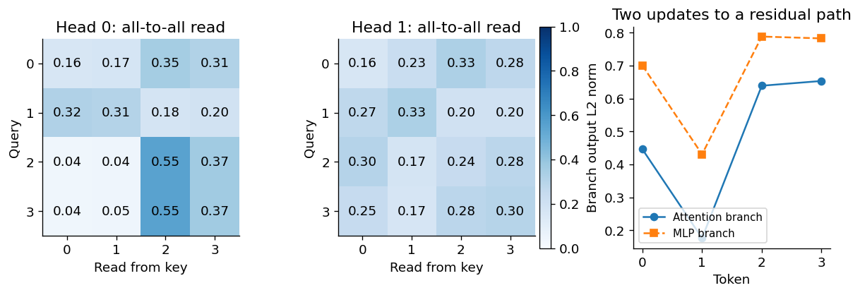
在这个计算里,每个 query 都可读取 4 个 key,因此没有语言自回归的“只能看过去”。注意力权重描述一次信息混合,不是因果解释,更不是物体重要性真值。
4. 一次改一个条件
- 像素条件:只把右下 patch 的最后一个像素增加 0.4;位置与全部权重不变。
- 位置条件:保持像素不变,只移除全部位置向量。
- 完全相同 token 对照:4 个 patch 内容完全相同且不加位置。预测四行 attention 和四个输出会怎样。
- 排列对照:不加位置时仅排列 token,预期输出按同样方式排列。这检验实现的置换等变关系,不检验真实视觉模型的识别能力。
这些是四个独立对照,不应合成一次“同时改变多项”的实验。
查看代码 · 单元 23
changed_image = image.copy(); changed_image[3,3] += .4
X_pixel = patchify(changed_image) @ W_patch + position
pixel_trace = encoder(X_pixel)
no_position = encoder(embedded)
identical_input = np.repeat(embedded[:1], 4, axis=0)
identical = encoder(identical_input)
permutation = np.array([2,0,3,1])
permuted = encoder(embedded[permutation])
assert np.allclose(identical['attention'], .25)
assert np.allclose(identical['output'], identical['output'][0])
assert np.allclose(permuted['output'], no_position['output'][permutation])
changes = {
    'one_pixel': {k: np.linalg.norm(pixel_trace[k]-trace[k],axis=-1).tolist() for k in ['input','projected_attention','residual1','mlp_output','output']},
    'remove_position': np.linalg.norm(no_position['output']-trace['output'],axis=-1).tolist(),
    'identical_attention_max_deviation_from_uniform': float(np.abs(identical['attention']-.25).max()),
    'permutation_max_error': float(np.abs(permuted['output']-no_position['output'][permutation]).max())}
print(json.dumps(changes,indent=2))
fig, ax=plt.subplots(figsize=(8,3.8))
for name, style in [('input','o--'),('projected_attention','s-'),('output','^-')]:
    ax.plot(range(4), changes['one_pixel'][name], style, label=name)
ax.set(xlabel='Token index',ylabel='L2 change',title='Change one pixel in patch 3; all weights fixed',xticks=range(4))
ax.legend(); fig.tight_layout(); fig.savefig(OUTPUT/'03-change-one-patch.png'); plt.show()
保存输出 · 2026-09-18 本地逐单元计算,非 Deepnote 云端运行
{
  "one_pixel": {
    "input": [
      0.0,
      0.0,
      0.0,
      0.36441734316577207
    ],
    "projected_attention": [
      0.13845143692262174,
      0.06075535944896897,
      0.10211094716003967,
      0.3623462524857455
    ],
    "residual1": [
      0.13845143692262177,
      0.06075535944896893,
      0.10211094716003964,
      0.241598612392958
    ],
    "mlp_output": [
      0.005507455494816578,
      0.1869619578853635,
      0.1485668531107396,
      0.368001638977608
    ],
    "output": [
      0.13750777740178868,
      0.17868250228813706,
      0.18240298330694946,
      0.5225156880808108
    ]
  },
  "remove_position": [
    0.4607686836719755,
    0.5561112107719021,
    0.30748062645628643,
    0.24410837570873786
  ],
  "identical_attention_max_deviation_from_uniform": 0.0,
  "permutation_max_error": 2.220446049250313e-16
}
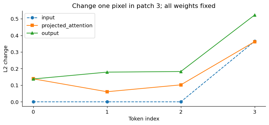
解释结果时分开两步: 残差直接把像素改动带到第 3 个 token;attention 让其他位置的读回也可能改变。逐 token MLP 自身不跨位置读数据,但它的输入已经含有 attention 交换的信息。因此不能看到多位置变化就说“MLP 自己做了空间通信”。
相同 token 对照给出均匀权重,是这个对称输入与固定模型的数学结果;并不是“没有位置编码就永远只能平均”。不相同的图块仍可产生不同的 Q、K。
5. 保留可核查结果,再提出你的反例
完整中间张量保存为 JSON 和 NPZ;CSV 每行对应一个 token 的变化。学生可以只改 image[3,3]、position 或某一个投影矩阵,然后运行全本。先写出预测、保持不动的条件,再观察与解释。
研究卡:如果输出变化很小,可能是 attention 变化小,也可能是输出投影抵消,或残差占比大。用哪些中间张量区分这些解释?怎样构造 attention 大幅变化而最终输出几乎不变的反例?不要把最终热图颜色当作答案。
查看代码 · 单元 28
import csv
artifact = {'kind':'exact_constructed_calculation_not_trained_model', 'seed':SEED,
            'environment':{'python':sys.version,'numpy':np.__version__,'platform':platform.platform()},
            'structure':{'norm':'pre-norm','heads':HEADS,'d_model':D,'d_head':DH,'d_ff':DFF,'epsilon':EPS,
                         'mask':'none','dropout':0,'gelu':'tanh approximation','class_token':False},
            'image':image.tolist(),'patches':patches.tolist(),'position':position.tolist(),
            'patch_projection':W_patch.tolist(),'weights':{k:v.tolist() for k,v in weights.items()},
            'trace':{k:v.tolist() for k,v in trace.items()},'changes':changes,
            'checks':{'manual_readback':True,'softmax_rows_sum_one':True,'residuals':True,
                      'identical_tokens_uniform':True,'no_position_permutation_equivariance':True}}
(OUTPUT/'results.json').write_text(json.dumps(artifact,indent=2),encoding='utf-8')
np.savez_compressed(OUTPUT/'tensors.npz', **trace, **weights, image=image, position=position, W_patch=W_patch)
with (OUTPUT/'token-changes.csv').open('w',newline='') as f:
    w=csv.writer(f); w.writerow(['token','input_l2_change','attention_branch_l2_change','output_l2_change'])
    for i in range(4): w.writerow([i]+[changes['one_pixel'][k][i] for k in ['input','projected_attention','output']])
print('Saved:', sorted(p.name for p in OUTPUT.iterdir()))
保存输出 · 2026-09-18 本地逐单元计算,非 Deepnote 云端运行
Saved: ['01-patches.png', '02-readback.png', '03-change-one-patch.png', 'results.json', 'tensors.npz', 'token-changes.csv']
来源与验证范围
来源:ViT 作者稿 v2,§3.1 / Eqs.2–3,用于图块投影、位置与 pre-norm encoder 的结构约定。参考图中的 scalar q/k/v 与本册双头完整层是两组计算例,不共享权重。
保存图与张量来自 2026-09-18 的本地逐单元计算,已核对手工读回、残差、相同 token 和排列对照;没有预训练或语义识别。页面上的保存输出可直接阅读,在自己的 Deepnote 副本运行时以实际新输出为准。
返回第二讲 · 后续 Attention 选读 · 网页阅读版与保存结果 · 下载 Lecture02-LAB09.ipynb · 课程导读