LAB 02 · 小 CNN 与图像平移
返回第二讲 · 图像平移与预测变化 · 第二讲导读与学习材料
结构与平移增强,分别改变了什么? 先读保存的四组结果,再跟踪同一张图前后的预测;这一段课堂活动无需重训。
| 本次想做什么 | 入口与操作 | 需要的准备 |
|---|---|---|
| 比较结构 × 增强 | 先读“既有实验的执行记录”,再看第5节图表与第6节失败样本 | 只读保存图即可 |
| 检查模型接口 | 文末“把旧 LeNet 与本次小 CNN 逐层对齐”;只改 FIRST_PADDING=2→0 |
独立代码块,PyTorch,无数据下载 |
| 检查标签怎样改变反馈 | 文末“交叉熵究竟把什么信号送回 logits”;只改 TRUE_CLASS=0→2 |
独立代码块,PyTorch,只求导 |
| 重新训练四组模型 | 第1–7节按顺序运行 | MNIST 文件、完整训练时间和独立结果目录 |
课堂先做一个可核对的判断。 比较 MLP 的有/无增强,再比较 CNN 的有/无增强:增强对右移表现的收益相同吗?接着查看原图准确率,检查收益有没有伴随取舍。不要用不同结构、不同增强的两格同时变化来归因。
运行边界。 第5、6节绘图代码使用第4节建立的 runs、predictions、trained_models;现有代码没有自动从缓存恢复这三组内存变量的分支。有 .pt 文件不等于可以直接跳跑第5、6节。只读保存结果请直接看图;要免训练加载固定模型观察响应与遮挡,进入 第二讲 LAB08。
推荐顺序:协议 → 四格对照 → 配对失败样本 → 任选一个独立短练。 完整训练是复算路径,不是阅读材料的前置条件。
2×2 的两条轴是 MLP/CNN × 无增强/随机平移增强。四组沿用同一数据划分、6 epochs、batch顺序与优化器;测试的是同一批原图和右移2像素图。同一结构的有/无增强组从相同初始化出发。
参数与每步计算没有配平,且只有一个训练随机种子。因此它回答这个训练预算下的观测,不提供普遍架构排名。
目标
在统一数据、优化预算与测试样本下,区分模型结构与训练增强的作用;保留参数量差异、单种子和裁切带来的解释边界。
既有实验的执行记录(沿用)
以下为本册保存的本地 CPU 四组运行:单 seed、各 6 epochs;四组均按最低干净验证损失选中第 6 轮。
| 模型 / 训练输入 | 原图正确 / 10,000 | 原图准确率 | 右移 2px 准确率 |
|---|---|---|---|
| MLP / no augmentation | 9211 | 92.11% | 66.39% |
| MLP + shift augmentation | 8994 | 89.94% | 84.21% |
| CNN / no augmentation | 9533 | 95.33% | 84.64% |
| CNN + shift augmentation | 9581 | 95.81% | 93.84% |
增强在本次 MLP 上改善位移表现,但降低了干净图像表现;CNN 的本次增强组两项都提高。这个取舍正是实验要揭示的结果,不能预设「增强一定全面改善」。这不是等计算比较:MLP/CNN 分别为 25,450/26,698 参数,每样本 Conv+Linear 前向 MAC 为 25,408/307,648。训练 seed 只有一个,尚不能据此报告统计显著性。
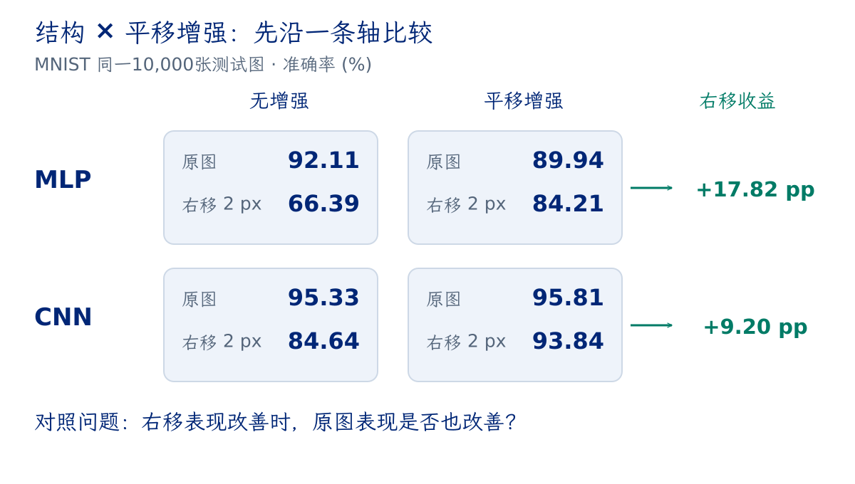
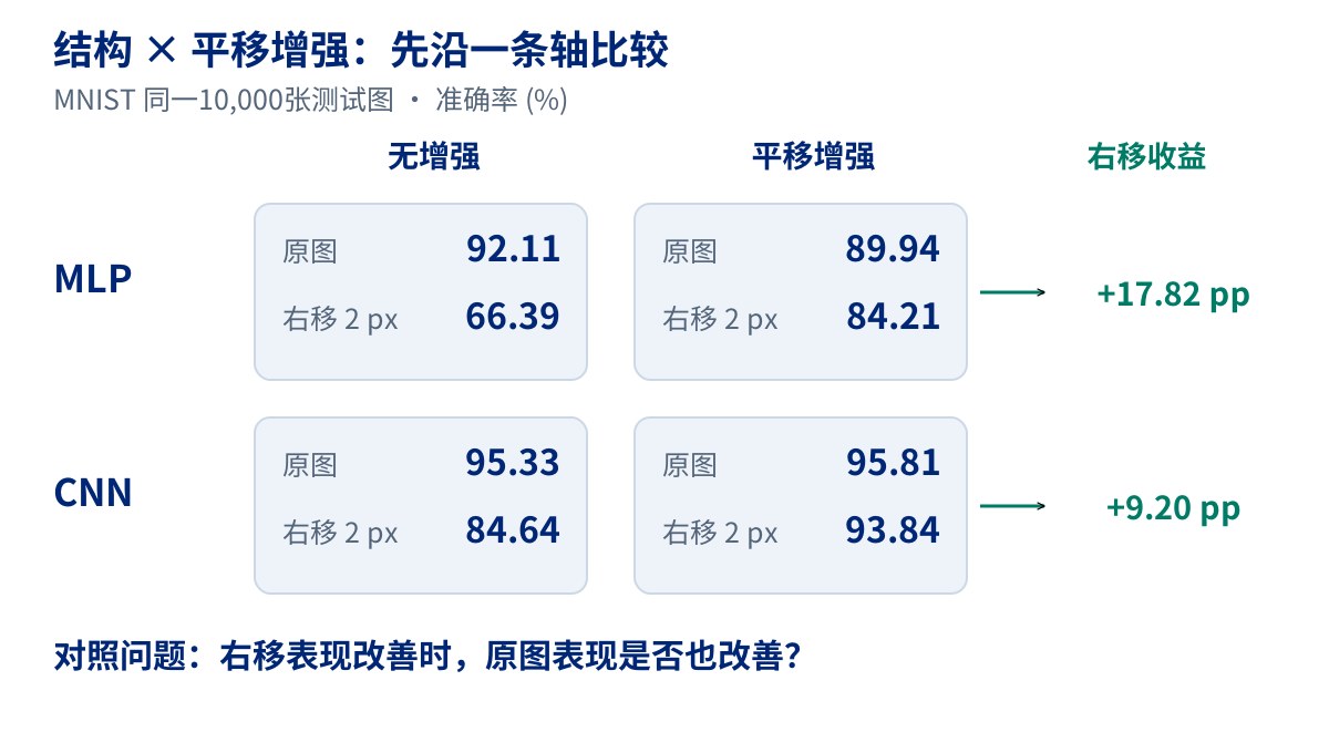
按行比较增强,按列比较结构。 先遮住右侧“增强收益”,根据两格的右移准确率自己计算;单位是百分点(pp)。再说出为什么 MLP 的原图表现使“增强全面改善”的说法不成立。
准备与使用
从头复算时本册会准备MNIST并训练四组模型;只读历史结果或运行文末独立小练习不需要这一训练流程。需要 Python 3.10+ 与 numpy matplotlib torch ipython;保存/检查 notebook 另需 nbformat matplotlib-inline。安装命令:
python -m pip install numpy matplotlib torch ipython nbformat matplotlib-inline
保存图与文末记录来自此前 Python 3.12 / PyTorch 2.14.0+cpu 的本地执行。你自己的运行环境版本由下一代码块打印;本次整理未重跑这些训练。图轴使用英文,正文提供中文读图说明。缺依赖时再安装,已有环境不必重复安装;课堂按开头任务入口运行,不必 Run all。
本材料改编自 Aston Zhang、Zachary C. Lipton、Mu Li、Alexander J. Smola 的 Dive into Deep Learning。D2L 正文 CC BY-SA 4.0,示例代码 modified MIT,许可随完整包 licenses/ 保存。我们补充多通道梯度、采样反例、受控实验、真实 PyTorch 状态语义;不要把教学小实现视为框架底层实现。
查看代码 · 单元 10
from pathlib import Path
import copy, hashlib, inspect, json, math, platform, time
import numpy as np
import matplotlib.pyplot as plt
import torch
from torch import nn
from torch.nn import functional as F
from IPython.display import display, Markdown

torch.manual_seed(20260921)
torch.set_num_threads(2)
torch.use_deterministic_algorithms(True)
OUT=Path('results'); OUT.mkdir(exist_ok=True)
FIG=Path('figures'); FIG.mkdir(exist_ok=True)
BLUE,GOLD,TEAL,RED='#002676','#FDB515','#00897B','#B83A3A'
plt.rcParams.update({'font.size':11,'axes.spines.top':False,'axes.spines.right':False,
                     'figure.dpi':110,'savefig.facecolor':'white'})
def savefig(fig,name):
    fig.savefig(FIG/f'{name}.png',dpi=160,bbox_inches='tight')
    fig.savefig(FIG/f'{name}.svg',bbox_inches='tight')
def table(headers,rows):
    display(Markdown('| '+' | '.join(headers)+' |\n| '+ ' | '.join(['---']*len(headers))+' |\n'+
                     '\n'.join('| '+' | '.join(map(str,row))+' |' for row in rows)))
print('PyTorch',torch.__version__,'/ Python',platform.python_version(),'/ device CPU')
1. 预先固定协议,测试结果不用于调参
标准 MNIST:从官方 60k train 按 NumPy seed 20260908 打乱,前 12k 训练,原 50k 之后的 10k 验证;官方 10k test 完全保留。四个原始 gzip 校验 MD5/SHA256,离线完整包包含它们。
四组均训练 6 epochs、batch 128、Adam 1e-3、初始化 seed 20260921,按干净 validation cross-entropy 最小选择 checkpoint。增强只发生在训练:每张图独立采样 dx,dy∈{-2,-1,0,1,2},零填充、裁切,不循环绕回。四组 batch 顺序相同,两个增强组的随机位移序列相同;同一结构的有/无增强组初始参数完全相同。
测试变换预先固定为向右 2 像素。它会裁去右侧像素;不是无信息损失的抽象群作用。本实验同时测原图表现、位移表现和成对预测变化。
查看代码 · 单元 13
SPLIT_SEED,MODEL_SEED=20260908,20260921
TRAIN_N,EPOCHS,BATCH_SIZE,LEARNING_RATE=12000,6,128,.001
查看代码 · 单元 14
import gzip, struct, urllib.request

# 读取完整标准 MNIST 文件;先用本地副本,没有时从 PyTorch 使用的公开镜像下载。
DATA = Path("data"); DATA.mkdir(exist_ok=True)
MNIST_FILES = {
    "train-images-idx3-ubyte.gz": "f68b3c2dcbeaaa9fbdd348bbdeb94873",
    "train-labels-idx1-ubyte.gz": "d53e105ee54ea40749a09fcbcd1e9432",
    "t10k-images-idx3-ubyte.gz": "9fb629c4189551a2d022fa330f9573f3",
    "t10k-labels-idx1-ubyte.gz": "ec29112dd5afa0611ce80d1b7f02629c",
}
data_identity = []
for filename, expected in MNIST_FILES.items():
    path = DATA / filename
    if not path.exists():
        url = "https://ossci-datasets.s3.amazonaws.com/mnist/" + filename
        try:
            with urllib.request.urlopen(url, timeout=60) as source:
                path.write_bytes(source.read())
        except Exception as exc:
            raise RuntimeError("MNIST 下载失败。请将课程材料包中 data/ 的四个 .gz 文件上传到项目 data/,再重跑。本实验不会退回伪造数据。") from exc
    raw = path.read_bytes()
    if hashlib.md5(raw).hexdigest() != expected:
        raise ValueError(f"MNIST 文件校验失败:{path},请重新取得该文件。")
    data_identity.append({"file":filename, "bytes":len(raw), "md5":expected,
                          "sha256":hashlib.sha256(raw).hexdigest()})

def read_idx(filename):
    with gzip.open(DATA / filename, "rb") as source:
        magic, n = struct.unpack(">II", source.read(8))
        if magic == 2051:
            h, w = struct.unpack(">II", source.read(8))
            assert (h, w) == (28, 28)
            return np.frombuffer(source.read(), np.uint8).reshape(n, 1, h, w).copy()
        assert magic == 2049
        return np.frombuffer(source.read(), np.uint8).reshape(n).copy()

raw_train = read_idx("train-images-idx3-ubyte.gz")
raw_train_y = read_idx("train-labels-idx1-ubyte.gz")
raw_test = read_idx("t10k-images-idx3-ubyte.gz")
raw_test_y = read_idx("t10k-labels-idx1-ubyte.gz")
assert raw_train.shape == (60000, 1, 28, 28) and raw_test.shape == (10000, 1, 28, 28)

# 沿用第一讲划分 seed;本次只从原先 50k train 取固定 12k 子集。
partition = np.random.default_rng(SPLIT_SEED).permutation(60000)
train_ids, val_ids = partition[:TRAIN_N], partition[50000:]
assert not set(train_ids).intersection(val_ids)
train_x = torch.tensor(raw_train[train_ids], dtype=torch.float32) / 255
train_y = torch.tensor(raw_train_y[train_ids], dtype=torch.long)
val_x = torch.tensor(raw_train[val_ids], dtype=torch.float32) / 255
val_y = torch.tensor(raw_train_y[val_ids], dtype=torch.long)
test_x = torch.tensor(raw_test, dtype=torch.float32) / 255
test_y = torch.tensor(raw_test_y, dtype=torch.long)
print(f"MNIST: train={len(train_y):,} / validation={len(val_y):,} / test={len(test_y):,}")
print("12k training labels:", np.bincount(raw_train_y[train_ids]).tolist())
2. 两个可读的模型,明确不是等参数 / 等计算
MLP 为 784→32→10;CNN 为 Conv(1→8)→pool→Conv(8→16)→pool→784→32→10。二者都输出 logits,cross_entropy 内部处理 log-softmax,不提前 softmax。
记录参数与每个样本前向 MAC(只统计 Conv/Linear 的乘加对,不把 ReLU、pool、内存流量计入)。相同 epoch 数控制了看数据的次数,没有控制 FLOPs 或 wall-clock。
查看代码 · 单元 17
from collections import OrderedDict
def make_model(kind):
    if kind=='MLP':
        return nn.Sequential(OrderedDict([('flatten',nn.Flatten()),('hidden',nn.Linear(784,32)),
                                         ('relu',nn.ReLU()),('logits',nn.Linear(32,10))]))
    return nn.Sequential(OrderedDict([
        ('conv1',nn.Conv2d(1,8,3,padding=1)),('relu1',nn.ReLU()),('pool1',nn.MaxPool2d(2)),
        ('conv2',nn.Conv2d(8,16,3,padding=1)),('relu2',nn.ReLU()),('pool2',nn.MaxPool2d(2)),
        ('flatten',nn.Flatten()),('hidden',nn.Linear(784,32)),('relu3',nn.ReLU()),('logits',nn.Linear(32,10))]))
model_info={}
for kind in ('MLP','CNN'):
    torch.manual_seed(MODEL_SEED);m=make_model(kind)
    v=torch.zeros(1,1,28,28);macs=0;shapes=[]
    for name,layer in m.named_children():
        v=layer(v);shapes.append([name,str(tuple(v.shape))])
        if isinstance(layer,nn.Conv2d):macs+=v.numel()*layer.in_channels*math.prod(layer.kernel_size)//layer.groups
        if isinstance(layer,nn.Linear):macs+=layer.in_features*layer.out_features
    model_info[kind]={'parameters':sum(p.numel() for p in m.parameters()),'conv_linear_macs':macs,'shapes':shapes}
assert model_info['CNN']['parameters']==26698
table(['Model','Parameters','Forward MACs / sample'],[[k,v['parameters'],v['conv_linear_macs']] for k,v in model_info.items()])
3. 把增强写成可检查的操作
位移增强不是对测试集做特化优化:训练覆盖水平与垂直的 25 个整数位移组合,而测试只使用预先固定的右移 2 像素。变换没有改变标签;但原始数字若贴边,裁切可能损失笔画。因此「标签应保持不变」是一项数据假设,需要看样本,而非任何变换都合法。
查看代码 · 单元 20
def translate(batch,dx,dy):
    result=torch.zeros_like(batch)
    H,W=batch.shape[-2:]
    x0,x1=max(0,-dx),min(W,W-dx)
    y0,y1=max(0,-dy),min(H,H-dy)
    result[:,:,y0+dy:y1+dy,x0+dx:x1+dx]=batch[:,:,y0:y1,x0:x1]
    return result

def augment(batch,generator):
    shifts=torch.randint(-2,3,(len(batch),2),generator=generator)
    result=torch.zeros_like(batch)
    for dx in range(-2,3):
        for dy in range(-2,3):
            mask=(shifts[:,0]==dx)&(shifts[:,1]==dy)
            if mask.any():result[mask]=translate(batch[mask],dx,dy)
    return result

shifted_test=translate(test_x,2,0)
assert torch.equal(shifted_test[:,:,:,2:],test_x[:,:,:,:-2])
assert shifted_test[:,:,:,:2].count_nonzero()==0
fig,axes=plt.subplots(2,6,figsize=(10,3.8))
sample_ids=[0,1,2,3,4,5]
for j,i in enumerate(sample_ids):
    for row,arr in enumerate([test_x,shifted_test]):
        axes[row,j].imshow(arr[i,0],cmap='gray',vmin=0,vmax=1);axes[row,j].axis('off')
        axes[row,j].set_title(f'id {i}, label {int(test_y[i])}' if row==0 else 'Right 2 px')
savefig(fig,'lab02-fixed-test-shift');plt.show()
保存结果|同一图的右移,不是另取一张图
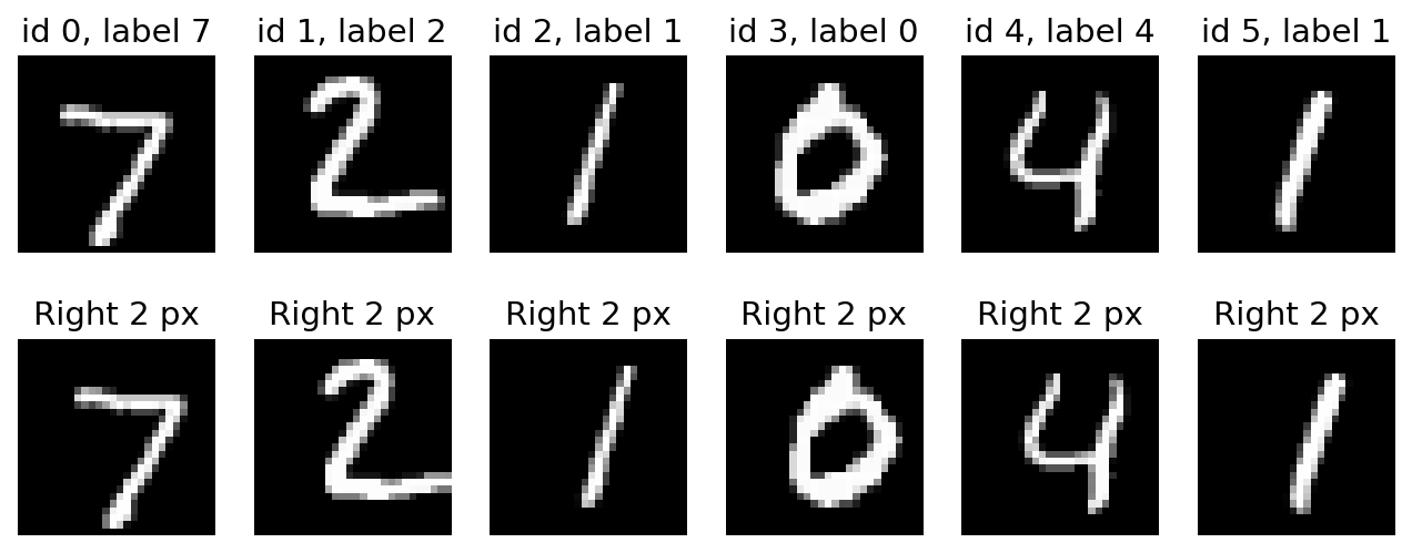
逐列对应相同 test ID,上行为原图,下行为右移2像素。先看左侧新增的零列,再检查右侧是否裁掉笔画。这里使用零填充/裁切,不是 roll 的循环绕回;后者会改变所检验的问题。
4. 真实训练四组:先用验证集选模型,再看测试
训练日志每个 epoch 仅打印一行。train_online_loss 在参数持续更新的过程中累计,验证损失在 epoch 末冻结参数上计算,二者测量时刻不同。不要仅凭训练/验证曲线间距判断过拟合。
即使增强影响干净验证损失的最佳 epoch,本协议仍统一以干净验证损失选模型,保持选择规则一致。可以另做增强验证集选择的实验,但应当提前另立协议,不能看测试结果后修改。
执行前停一下。 下一个代码块会真实训练四组模型,并将检查点写入 results/;第7节还会保存协议 JSON。若今天只讨论课件曲线,请看后面的保存图,不运行这个训练块。若要复算,先在自己的项目副本中保留旧结果,并从准备、协议、数据、模型与增强依次运行;不能只运行绘图单元。
查看代码 · 单元 24
# 将来源记录绑定到这次真实训练与保存的文件,防止与旧 report 混用。
assert TRAIN_N==len(train_y)==len(train_ids)
assert torch.equal(train_x,torch.tensor(raw_train[train_ids],dtype=torch.float32)/255)
assert torch.equal(train_y,torch.tensor(raw_train_y[train_ids],dtype=torch.long))
assert torch.equal(val_x,torch.tensor(raw_train[val_ids],dtype=torch.float32)/255)
assert torch.equal(val_y,torch.tensor(raw_train_y[val_ids],dtype=torch.long))
training_source_protocol={
    'split_seed':int(SPLIT_SEED),'train_n':len(train_ids),'validation_n':len(val_ids),
    'partition_sha256':hashlib.sha256(partition.tobytes()).hexdigest(),
    'train_ids_sha256':hashlib.sha256(train_ids.tobytes()).hexdigest(),
    'validation_ids_sha256':hashlib.sha256(val_ids.tobytes()).hexdigest(),
    'files':copy.deepcopy(data_identity)}
checkpoint_provenance={}

@torch.no_grad()
def evaluate(model,x,y,batch_size=512):
    model.eval()
    logits=torch.cat([model(x[i:i+batch_size]) for i in range(0,len(x),batch_size)])
    pred=logits.argmax(1);correct=int((pred==y).sum())
    return {'n':len(y),'correct':correct,'accuracy':correct/len(y),
            'loss':float(F.cross_entropy(logits,y))},pred

runs={};trained_models={};predictions={};initial_hashes={}
for kind in ('MLP','CNN'):
    for use_aug in (False,True):
        label=kind+(' + shift augmentation' if use_aug else ' / no augmentation')
        torch.manual_seed(MODEL_SEED);model=make_model(kind)
        init_hash=hashlib.sha256(b''.join(p.detach().numpy().tobytes() for p in model.parameters())).hexdigest()
        initial_hashes[label]=init_hash
        optimizer=torch.optim.Adam(model.parameters(),lr=LEARNING_RATE)
        shuffle=torch.Generator().manual_seed(MODEL_SEED+1)
        augmentation_rng=torch.Generator().manual_seed(MODEL_SEED+2)
        history=[];best_loss=float('inf');best_state=None
        start=time.perf_counter()
        for epoch in range(1,EPOCHS+1):
            model.train();order=torch.randperm(TRAIN_N,generator=shuffle);total_loss=0.
            for idx in order.split(BATCH_SIZE):
                xb=augment(train_x[idx],augmentation_rng) if use_aug else train_x[idx]
                optimizer.zero_grad(set_to_none=True)
                loss=F.cross_entropy(model(xb),train_y[idx]);loss.backward();optimizer.step()
                total_loss+=float(loss.detach())*len(idx)
            val,_=evaluate(model,val_x,val_y)
            history.append({'epoch':epoch,'train_online_loss':total_loss/TRAIN_N,
                            'val_loss':val['loss'],'val_accuracy':val['accuracy']})
            if val['loss']<best_loss:
                best_loss=val['loss'];best_state=copy.deepcopy(model.state_dict());best_epoch=epoch
            print(f'{label} | epoch {epoch}: val loss={val["loss"]:.4f}, val acc={val["accuracy"]:.2%}')
        seconds=time.perf_counter()-start
        model.load_state_dict(best_state)
        clean,p0=evaluate(model,test_x,test_y);shifted,p1=evaluate(model,shifted_test,test_y)
        original_ok=p0==test_y;shifted_ok=p1==test_y
        transitions={'correct_to_correct':int((original_ok&shifted_ok).sum()),
                     'correct_to_wrong':int((original_ok&~shifted_ok).sum()),
                     'wrong_to_correct':int((~original_ok&shifted_ok).sum()),
                     'wrong_to_wrong':int((~original_ok&~shifted_ok).sum())}
        runs[label]={'architecture':kind,'augmentation':use_aug,'parameters':model_info[kind]['parameters'],
                     'conv_linear_macs':model_info[kind]['conv_linear_macs'],'history':history,
                     'selected_epoch':best_epoch,'seconds':seconds,'initial_state_sha256':init_hash,
                     'clean':clean,'right_2px':shifted,'prediction_changed':int((p0!=p1).sum()),'paired':transitions}
        trained_models[label]=model;predictions[label]=(p0,p1)
        checkpoint_name=kind.lower()+('-aug' if use_aug else '-plain')+'-state.pt'
        checkpoint_path=OUT/checkpoint_name
        torch.save(best_state,checkpoint_path)
        checkpoint_provenance[checkpoint_name]={
            'run_label':label,'sha256':hashlib.sha256(checkpoint_path.read_bytes()).hexdigest(),
            'source_protocol':copy.deepcopy(training_source_protocol)}
for kind in ('MLP','CNN'):
    hashes=[v for k,v in initial_hashes.items() if k.startswith(kind)]
    assert len(set(hashes))==1
print('All four runs complete; identical initial weights confirmed within each architecture.')
5. 观测:2×2 结果、训练曲线与交互项
准确率是同一 10k 样本上的比例;下面同时给出 clean/right-shift 数值和 correct→wrong 转移。结构效应可能依赖增强策略,增强效应也可能依赖结构。用百分点差的差表达这个交互,不能把它解释为已排除种子/预算影响的普遍因果律。
与主讲曲线对应的统计口径。 CNN/无增强的历史记录按最小 val_loss 选择 epoch 6,验证交叉熵为 0.1610109955072403。train_online_loss 累计一轮中边更新参数边计算的训练损失,val_loss 则在轮末固定模型评估;二者不在同一参数时刻统计。这次两条曲线均下降,不能只按曲线高低判定过拟合。原始记录见 LAB02 结果 JSON。本轮只重绘已保存的 CSV/JSON,没有重新训练;本节四组实验和下面的保存输出继续保留原身份。
查看代码 · 单元 27
labels=list(runs)
table(['Condition','Selected epoch','Clean correct / 10000','Clean %','Right 2px %','Correct → wrong'],[
    [k,v['selected_epoch'],v['clean']['correct'],f"{100*v['clean']['accuracy']:.2f}",
     f"{100*v['right_2px']['accuracy']:.2f}",v['paired']['correct_to_wrong']] for k,v in runs.items()])
fig,axes=plt.subplots(1,2,figsize=(12,4))
pos=np.arange(4);width=.35
axes[0].bar(pos-width/2,[100*runs[k]['clean']['accuracy'] for k in labels],width,label='Clean',color=BLUE)
axes[0].bar(pos+width/2,[100*runs[k]['right_2px']['accuracy'] for k in labels],width,label='Right 2 px',color=TEAL)
axes[0].set(xticks=pos,xticklabels=['MLP','MLP + aug','CNN','CNN + aug'],ylabel='Accuracy (%)',ylim=(0,120),yticks=[0,20,40,60,80,100],title='Same 10,000 test images');axes[0].legend(loc='upper left',ncol=2)
for i,k in enumerate(labels):
    for offset,metric in [(-width/2,'clean'),(width/2,'right_2px')]:
        v=100*runs[k][metric]['accuracy'];axes[0].text(i+offset,v+1,f'{v:.1f}',ha='center',fontsize=9)
for k,color,marker in zip(labels,[BLUE,TEAL,RED,'#6957A0'],['o','s','^','D']):
    axes[1].plot([v['epoch'] for v in runs[k]['history']],[v['val_loss'] for v in runs[k]['history']],marker=marker,color=color,label=k.replace('shift augmentation','aug').replace(' / no augmentation',''))
axes[1].set(xlabel='Epoch',ylabel='Validation cross-entropy',title='Clean validation selects each checkpoint');axes[1].legend(fontsize=8)
fig.tight_layout();savefig(fig,'lab02-controlled-2x2');plt.show()
shift_acc=[100*runs[k]['right_2px']['accuracy'] for k in labels]
interaction_pp=(shift_acc[3]-shift_acc[2])-(shift_acc[1]-shift_acc[0])
display(Markdown(f'本次运行:MLP 的增强收益为 **{shift_acc[1]-shift_acc[0]:+.2f} pp**,CNN 为 **{shift_acc[3]-shift_acc[2]:+.2f} pp**;差的差(CNN − MLP)为 **{interaction_pp:+.2f} pp**。这是单 seed 的观测,不附会统计显著性。'))
保存结果|先选择检查点,再比较测试
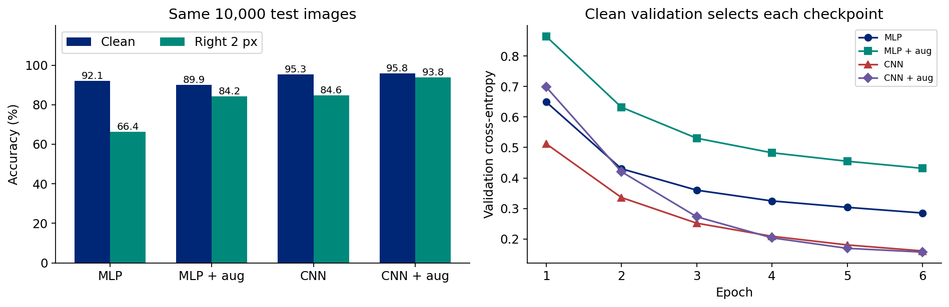
左图比较同一10,000张测试图;每组两柱分别是原图与右移2像素。右图是用于选择检查点的干净验证交叉熵,越低越好。先在同一结构内读两种训练条件,再跨结构比较;不要把右图的验证选择与左图的最终测试混为一次调参。
6. 配对检查:哪张图从对变错?
准确率相同也可能对应完全不同的预测。下面从 CNN 无增强组中按官方 test index 升序取最早 6 个「原图正确、右移错误」的样本,不人为挑选视觉最戏剧性的例子。若没有符合条件的样本,代码如实说明并显示前 6 个样本。
第一层激活从已训练网络实际提取,展示同一张图平移前后。颜色响应强不等于某通道有稳定语义,也不能把激活图解释为因果归因。
查看代码 · 单元 31
label='CNN / no augmentation';p0,p1=predictions[label]
ids=torch.where((p0==test_y)&(p1!=test_y))[0][:6]
selection='first six test indices where clean is correct and shifted is wrong'
if not len(ids):ids=torch.arange(6);selection='no clean-correct/shift-wrong case; first six test indices'
fig,axes=plt.subplots(2,len(ids),figsize=(max(6,len(ids)*1.6),3.7),squeeze=False)
for j,i in enumerate(ids.tolist()):
    axes[0,j].imshow(test_x[i,0],cmap='gray');axes[0,j].set_title(f'id {i}\ny={int(test_y[i])}, p={int(p0[i])}',fontsize=10)
    axes[1,j].imshow(shifted_test[i,0],cmap='gray');axes[1,j].set_title(f'Shifted: p={int(p1[i])}',fontsize=10)
    for ax in axes[:,j]:ax.axis('off')
fig.tight_layout();savefig(fig,'lab02-paired-failures');plt.show()
保存结果|从总体比例回到同一张图
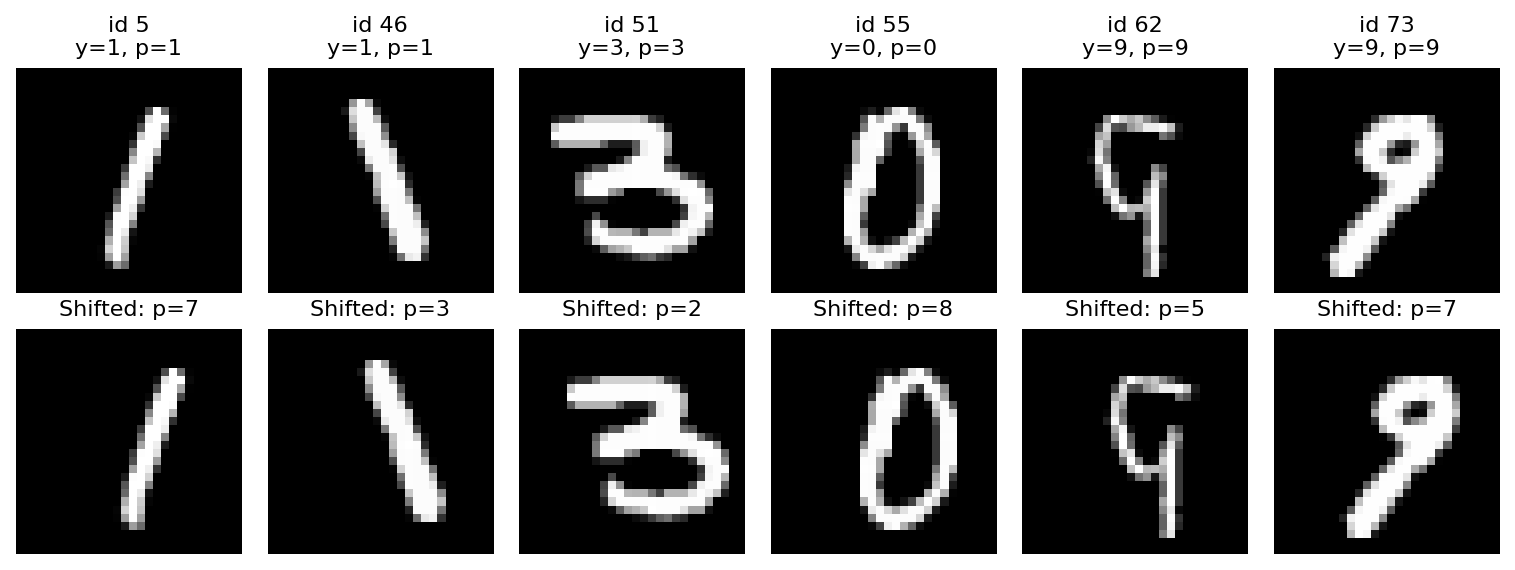
先选一列,指出 y(真实类别)、上方 p(原图预测)和下方 p(右移预测)。选样规则是 CNN 无增强组中按 test ID 升序最早6个“正确→错误”,不是随机代表样本。因此这6列用于解释失败现象,不能拿来重新估计总体准确率。
查看代码 · 单元 33
chosen=int(ids[0]);m=trained_models[label]
with torch.no_grad():a0=F.relu(m.conv1(test_x[chosen:chosen+1]))[0];a1=F.relu(m.conv1(shifted_test[chosen:chosen+1]))[0]
fig,axes=plt.subplots(2,8,figsize=(13,3.8));limit=float(torch.cat([a0,a1]).max())
for c in range(8):
    for row,a in enumerate([a0,a1]):
        axes[row,c].imshow(a[c],cmap='magma',vmin=0,vmax=limit);axes[row,c].axis('off');axes[row,c].set_title(f'Channel {c}')
fig.suptitle(f'Actual first-layer ReLU activations: test index {chosen}; top clean, bottom right 2px')
savefig(fig,'lab02-actual-activations');plt.show()
保存结果|移动的响应与变化的类别预测
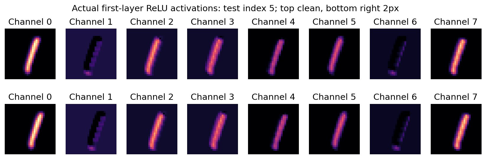
先固定一列通道比较上下两行:上为原图,下为右移2像素,全图用统一色标。响应跟着移动与最终类别保持不变是两个问题;前者不能替后者作答。继续做干预请用 第二讲 LAB08 · 从真实响应到遮挡对照。
7. 结论范围与可复现记录
能支持:本次固定数据/优化预算下,结构、增强与平移表现的关系;同一模型在同一批图上的配对变化。
不能支持:所有 CNN 的平移不变性、结构单独解释全部提升、一个 seed 的统计显著性、MNIST 结果外推 ImageNet/科学数据。进一步研究应运行多个种子,报告均值/离散程度,并考虑等参数、等计算或各自合理调参的比较;这些分别回答不同问题。
下面保存原始协议、文件身份、每轮验证记录与四份最佳参数。checkpoint 仅由验证集选择,test 没有参与训练或选择。
查看代码 · 单元 37
# 只保存本轮训练时登记的身份;不替换或补签未知文件。
if 'checkpoint_provenance' not in globals() or not checkpoint_provenance:
    raise RuntimeError('请先运行第4节训练单元,再保存本轮结果与模型身份。')
for checkpoint_name,identity in checkpoint_provenance.items():
    path=OUT/checkpoint_name
    if not path.is_file() or hashlib.sha256(path.read_bytes()).hexdigest()!=identity['sha256']:
        raise RuntimeError('模型文件与本轮训练登记不一致:'+str(path)+';请重新运行第4节,不能给混用文件补签。')
    saved_state=torch.load(path,map_location='cpu',weights_only=True)
    live_state=trained_models[identity['run_label']].state_dict()
    if set(saved_state)!=set(live_state) or any(not torch.equal(saved_state[k],live_state[k].cpu()) for k in saved_state):
        raise RuntimeError('内存模型与本轮保存文件不一致,请重新运行第4节。')
assert SPLIT_SEED==training_source_protocol['split_seed']
assert TRAIN_N==training_source_protocol['train_n']
assert hashlib.sha256(train_ids.tobytes()).hexdigest()==training_source_protocol['train_ids_sha256']
assert hashlib.sha256(val_ids.tobytes()).hexdigest()==training_source_protocol['validation_ids_sha256']

summary={'experiment':'Controlled 2x2: MLP/CNN x no augmentation/random integer translation',
 'execution':'all four runs executed in the current Python environment on CPU; single seed; no synthetic fallback',
 'environment':{'python':platform.python_version(),'torch':torch.__version__,'numpy':np.__version__,'torch_threads':torch.get_num_threads(),'deterministic_algorithms':torch.are_deterministic_algorithms_enabled()},
 'protocol':{'train_n':TRAIN_N,'validation_n':len(val_y),'test_n':len(test_y),'split_seed':SPLIT_SEED,
             'model_seed':MODEL_SEED,'shuffle_seed':MODEL_SEED+1,'augmentation_seed':MODEL_SEED+2,
             'epochs':EPOCHS,'batch_size':BATCH_SIZE,'optimizer':'Adam','learning_rate':LEARNING_RATE,
             'selection':'minimum clean validation cross-entropy; test not used',
             'train_augmentation':'independent per-image dx,dy uniform integers [-2,2], zero-fill/crop',
             'test_transform':'fixed right 2 px, zero-fill left and crop right',
             'split':f'NumPy permutation; first {TRAIN_N} train, positions 50000:60000 validation; official test',
             'partition_sha256':hashlib.sha256(partition.tobytes()).hexdigest(),
             'train_ids_sha256':hashlib.sha256(train_ids.tobytes()).hexdigest(),'files':data_identity},
 'models':model_info,'runs':runs,'shift_augmentation_interaction_pp':interaction_pp,
 'failure_examples':{'selection':selection,'test_indices':ids.tolist(),'activation_example':chosen},
 'limitations':['single seed','architectures have different parameters and compute','MNIST only','cropping may remove information']}
summary['checkpoint_provenance']=copy.deepcopy(checkpoint_provenance)
(OUT/'lab02-results.json').write_text(json.dumps(summary,indent=2))
print('Saved results/lab02-results.json and four selected model states.')
可选深读:怎样手算2×2效应
口径:四组都在同一组10000张右移2像素测试图上计算准确率。下面的pp表示百分点;先在各结构内计算“有增强减无增强”,再比较这两个增益。
MLP:84.21% − 66.39% = 17.82 pp;CNN:93.84% − 84.64% = 9.20 pp。两种结构在本次运行中都受益于平移增强。
交互差分按CNN减MLP定义:(93.84 − 84.64) − (84.21 − 66.39) = -8.62 pp。它描述的是本次实验中增强增益对结构的依赖,不是说增强对CNN有害。
这里只有一个随机种子。该差分没有给出跨训练种子的置信区间;高起点与准确率上限也可能影响百分点增益,因此不能据此断言两种先验的普遍替代关系。
预算边界:MLP与CNN每个样本的Conv/Linear MAC分别为25408与307648,后者约 12.11倍;相同epoch数并不等于相同计算预算。这里回答固定训练轮数下的观测,后续可再做等计算对照。
协议与来源沿革
历次备课记录与原数值表保留在。本实验使用前文明确的当前协议与模型身份;历史数值不与新运行合并。
返回 CLS 00 · 第二讲导读
历史实验再读 1 · 把旧 LeNet 与本次小 CNN 逐层对齐
先预测。 本 LAB 已给出当前 MLP/CNN 的结构与实测训练。本节补上旧课程的 LeNet 接口:同为 1×28×28 输入,为什么旧课 flatten 后是 400 维,本次 CNN 是 784 维?两次平均池化或最大池化之前的卷积分别改变了什么?先手算两条空间尺寸链。
修改参数再运行。 默认复现旧课的首层 padding=2;再改为 FIRST_PADDING=0,预测 flatten 维数与全连接参数量。INPUT_SIDE 也可从 28 改为 32。为让比较仍能运行,代码按实际卷积输出维数构造首个 Linear;因此替代设置是明确的结构变体,不是未改动的旧 LeNet。
历史来源与数据身份。 Spring26 Lecture3-2_lenet:project 03ca31da-8b5e-4562-82d0-0898f6eb7b7a,notebook 246394240a4f4eb0a30215bbe9c9492a;Fall25 Lecture4-6_lenet:project f60a1775-066c-48b1-a0c1-181c392044b6,notebook 300b831fe14e49d7a47daf0763be5d2d。旧课采用 Fashion-MNIST,而本 LAB 前面的实际四组实验使用 MNIST。本段仅复用旧课/D2L 教学 LeNet 的结构及逐层 shape 追踪,增加与当前 CNN 的参数对照;输入是零张量,不加载任何数据、不训练、不比较准确率。这是旧课教学实现,并非逐细节还原原始 LeNet-5 论文。
查看代码 · 单元 49
import torch
from torch import nn
from collections import OrderedDict

torch.set_num_threads(2)
INPUT_SIDE, FIRST_PADDING = 28, 2  # 再试:28, 0;或 32, 2
assert INPUT_SIDE in (28, 32) and FIRST_PADDING in (0, 2)
probe = torch.zeros(1, 1, INPUT_SIDE, INPUT_SIDE)
with torch.random.fork_rng(devices=[]):
    torch.manual_seed(26)
    old_features = nn.Sequential(OrderedDict([
        ('conv1', nn.Conv2d(1, 6, 5, padding=FIRST_PADDING)), ('sigmoid1', nn.Sigmoid()),
        ('avgpool1', nn.AvgPool2d(2)), ('conv2', nn.Conv2d(6, 16, 5)),
        ('sigmoid2', nn.Sigmoid()), ('avgpool2', nn.AvgPool2d(2)),
    ]))
    current_features = nn.Sequential(OrderedDict([
        ('conv1', nn.Conv2d(1, 8, 3, padding=1)), ('relu1', nn.ReLU()),
        ('maxpool1', nn.MaxPool2d(2)), ('conv2', nn.Conv2d(8, 16, 3, padding=1)),
        ('relu2', nn.ReLU()), ('maxpool2', nn.MaxPool2d(2)),
    ]))
    with torch.no_grad():
        old_width = old_features(probe).numel()
        current_width = current_features(probe).numel()
    old = nn.Sequential(OrderedDict(list(old_features.named_children()) + [
        ('flatten', nn.Flatten()), ('fc1', nn.Linear(old_width, 120)), ('sigmoid3', nn.Sigmoid()),
        ('fc2', nn.Linear(120, 84)), ('sigmoid4', nn.Sigmoid()), ('logits', nn.Linear(84, 10)),
    ]))
    current = nn.Sequential(OrderedDict(list(current_features.named_children()) + [
        ('flatten', nn.Flatten()), ('hidden', nn.Linear(current_width, 32)),
        ('relu3', nn.ReLU()), ('logits', nn.Linear(32, 10)),
    ]))

HISTORY_RESULT = {}
for name, model, width in [('Historical teaching LeNet', old, old_width), ('Current LAB02 CNN', current, current_width)]:
    value, rows = probe, []
    print('\n' + name)
    print(f"{'layer':<14} {'output shape':<22} {'parameters':>10}")
    with torch.no_grad():
        for layer_name, layer in model.named_children():
            value = layer(value)
            count = sum(p.numel() for p in layer.parameters())
            rows.append({'layer': layer_name, 'shape': list(value.shape), 'parameters': count})
            print(f'{layer_name:<14} {str(tuple(value.shape)):<22} {count:>10,}')
    assert tuple(value.shape) == (1, 10)
    total = sum(p.numel() for p in model.parameters())
    print('Flatten width:', width, '| total parameters:', total)
    HISTORY_RESULT[name] = {'flatten_width': width, 'parameters': total, 'layers': rows}
if (INPUT_SIDE, FIRST_PADDING) == (28, 2):
    assert (old_width, current_width) == (400, 784)
    assert HISTORY_RESULT['Historical teaching LeNet']['parameters'] == 61706
    assert HISTORY_RESULT['Current LAB02 CNN']['parameters'] == 26698
默认结果。 旧课空间尺寸为 28→28→14→10→5,flatten 为 16×5×5=400;当前 CNN 为 28→28→14→14→7,flatten 为 16×7×7=784。旧课教学 LeNet 共 61,706 参数,当前 CNN 共 26,698;参数最多的层可直接从表中定位。
讨论边界。 LeNet 的 flatten 更窄,却不代表总参数更少:后面的隐藏宽度也参与账单。改变 padding 还改变边界信息与首个 Linear 的输入尺寸;不能只看参数数目就推断准确率或计算成本。这里没有运行 Fashion-MNIST,也没有用未训练的 logits 作分类证据。若要比较泛化,需另立同数据、选择规则与预算清楚的训练协议。
历史实验再读 2 · 交叉熵究竟把什么信号送回 logits?
先预测。 本 LAB 已正确地把 logits 交给 cross_entropy,但尚未直接核对每个类别的反馈。固定三类分数 [2,1,0]:当真实类别从 0 改为 2,哪一个梯度应为负?给所有分数同时加 1000,概率、损失和梯度应改变吗?如果先 softmax 再交给 cross_entropy,算的还是同一个目标吗?
修改参数再运行。 默认后再试 TRUE_CLASS=2, SCALE=3.0, COMMON_SHIFT=-1000.0。观察每类的概率、p−one_hot(y)、autograd 梯度,以及错误重复 softmax 的梯度。SCALE 先决定本次分数;表中导数针对这些已缩放的 logits。只求导,不做优化器更新。
历史来源与改写。 Spring26 Lecture2-3_softmax-regression,project f8d9c543-5a2a-4932-9218-b83425e7d06f,notebook 6bc3ba9a8a4b4e4d9088a39c48a9af09。继承旧课“CrossEntropyLoss 前为何不再加 Softmax”的问题和 logits 接口;本次新写可手算的三类 autograd 核对,移除数据加载、Fashion-MNIST/FakeData 回退及训练过程。与前面 MNIST 四组实验的准确率分开解读。
查看代码 · 单元 53
import torch
from torch.nn import functional as F

TRUE_CLASS, SCALE, COMMON_SHIFT = 0, 1.0, 1000.0  # 再试:2, 3.0, -1000.0
assert TRUE_CLASS in (0, 1, 2) and 0 < SCALE <= 10
z = (torch.tensor([[2., 1., 0.]], dtype=torch.float64) * SCALE).requires_grad_()
y = torch.tensor([TRUE_CLASS], dtype=torch.long)
loss = F.cross_entropy(z, y)
grad, = torch.autograd.grad(loss, z)
p = z.detach().softmax(dim=1)
manual = p - F.one_hot(y, num_classes=3).to(p.dtype)
torch.testing.assert_close(grad, manual)

shifted = (z.detach() + COMMON_SHIFT).requires_grad_()
shifted_loss = F.cross_entropy(shifted, y)
shifted_grad, = torch.autograd.grad(shifted_loss, shifted)
torch.testing.assert_close(shifted.detach().softmax(1), p)
torch.testing.assert_close(shifted_loss, loss)
torch.testing.assert_close(shifted_grad, grad)

wrong_z = z.detach().clone().requires_grad_()
wrong_loss = F.cross_entropy(wrong_z.softmax(dim=1), y)
wrong_grad, = torch.autograd.grad(wrong_loss, wrong_z)
print(f"{'class':<7} {'logit':>8} {'p':>10} {'p-target':>12} {'autograd':>12} {'double-softmax grad':>20}")
for c in range(3):
    print(f'{c:<7} {z.detach()[0,c].item():8.3f} {p[0,c].item():10.6f} '
          f'{manual[0,c].item():12.6f} {grad[0,c].item():12.6f} {wrong_grad[0,c].item():20.6f}')
HISTORY_RESULT = {
    'true_class': TRUE_CLASS,
    'correct_ce': float(loss.detach()),
    'double_softmax_ce': float(wrong_loss.detach()),
    'manual_grad_max_error': float((grad-manual).abs().max()),
    'shift_loss_gap': float((shifted_loss.detach()-loss.detach()).abs()),
    'shift_grad_max_gap': float((shifted_grad-grad).abs().max()),
    'double_softmax_grad_max_gap': float((wrong_grad-grad).abs().max()),
    'gradient_sum': float(grad.sum()),
}
print('Checks:', HISTORY_RESULT)
默认核对。 概率约为 [0.665241,0.244728,0.090031],对真实类 0 的梯度约为 −0.334759,另外两项为正。梯度下降因此提高真实类分数、降低其他类分数。三项梯度的和约为 0,呼应共同平移不改变此目标。正确交叉熵约为 0.407606;重复 softmax 计算的是另一个目标,数值和回传梯度均不同。
讨论边界。 “梯度符号正确”不保证整体网络在任意学习率下变好;链式法则还要经过模型参数。SCALE 改变分数差,因此可改变置信度与梯度;COMMON_SHIFT 不改变分数差。这个例子不是校准评估,也不证明更高置信度更可靠。请解释:为什么直接计算 exp(1002) 容易溢出,而框架的稳定交叉熵仍可核对?